7 Lineare Regression
7.1 Packages
library(tidyverse)7.2 Datensatz Deskription
starwars <- starwars7.2.1 Beschreibung
# Augenfarbe ~ Masse
starwars %>%
  group_by(eye_color) %>%
  summarize(
    avg_mass = mean(mass, na.rm = T)
  )
## # A tibble: 15 × 2
## eye_color avg_mass
## <chr> <dbl>
## 1 black 76.3
## 2 blue 86.5
## 3 blue-gray 77
## 4 brown 66.1
## 5 dark NaN
## 6 gold NaN
## 7 green, yellow 159
## 8 hazel 66
## 9 orange 282.
## 10 pink NaN
## 11 red 81.4
## 12 red, blue NaN
## 13 unknown 31.5
## 14 white 48
## 15 yellow 81.1# 5-Punkte (nach Gewicht)
starwars %>%
group_by(gender) %>%
filter(!is.na(height)) %>%
summarize(
min_height = min(height),
q1_height = quantile(height,0.25),
med_height = quantile(height,0.5),
q3_height = quantile(height, 0.75),
max_height = max(height)
)## # A tibble: 3 × 6
## gender min_height q1_height med_height q3_height
## <chr> <int> <dbl> <dbl> <dbl>
## 1 feminine 96 162. 166. 172
## 2 masculine 66 171. 183 193
## 3 <NA> 178 180. 183 183
## # … with 1 more variable: max_height <int>7.2.2 Visualisieren
#erstmal eindeutschen
starwars %>%
  mutate(gender = fct_recode(gender,
    "Männlich" = "masculine",
    "Weiblich" = "feminine",
    "nichts" = "NA"
  )) %>%
  ggplot(aes(height, gender)) +
    geom_boxplot(na.rm = T) +
    geom_point(stat= "summary", fun = "mean", color = "red") +
    xlab("Größe in cm")+
    ylab("Geschlecht") +
    ggtitle("Boxplot der Größenverteilung nach Geschlecht")
## Warning: Unknown levels in `f`: NA## Warning: Removed 6 rows containing non-finite values
## (stat_summary).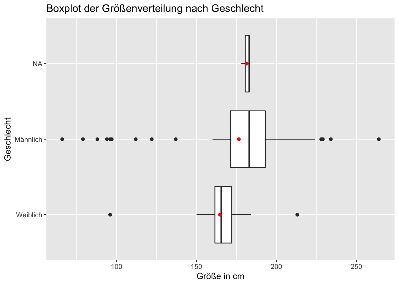
7.3 Regressionsanalyse (explorativ)
diamonds <- diamonds

summary(diamonds)
## carat cut color
## Min. :0.2000 Fair : 1610 D: 6775
## 1st Qu.:0.4000 Good : 4906 E: 9797
## Median :0.7000 Very Good:12082 F: 9542
## Mean :0.7979 Premium :13791 G:11292
## 3rd Qu.:1.0400 Ideal :21551 H: 8304
## Max. :5.0100 I: 5422
## J: 2808
## clarity depth table
## SI1 :13065 Min. :43.00 Min. :43.00
## VS2 :12258 1st Qu.:61.00 1st Qu.:56.00
## SI2 : 9194 Median :61.80 Median :57.00
## VS1 : 8171 Mean :61.75 Mean :57.46
## VVS2 : 5066 3rd Qu.:62.50 3rd Qu.:59.00
## VVS1 : 3655 Max. :79.00 Max. :95.00
## (Other): 2531
## price x y
## Min. : 326 Min. : 0.000 Min. : 0.000
## 1st Qu.: 950 1st Qu.: 4.710 1st Qu.: 4.720
## Median : 2401 Median : 5.700 Median : 5.710
## Mean : 3933 Mean : 5.731 Mean : 5.735
## 3rd Qu.: 5324 3rd Qu.: 6.540 3rd Qu.: 6.540
## Max. :18823 Max. :10.740 Max. :58.900
##
## z
## Min. : 0.000
## 1st Qu.: 2.910
## Median : 3.530
## Mean : 3.539
## 3rd Qu.: 4.040
## Max. :31.800
## diamonds %>%
ggplot(aes(carat,price)) +
geom_point()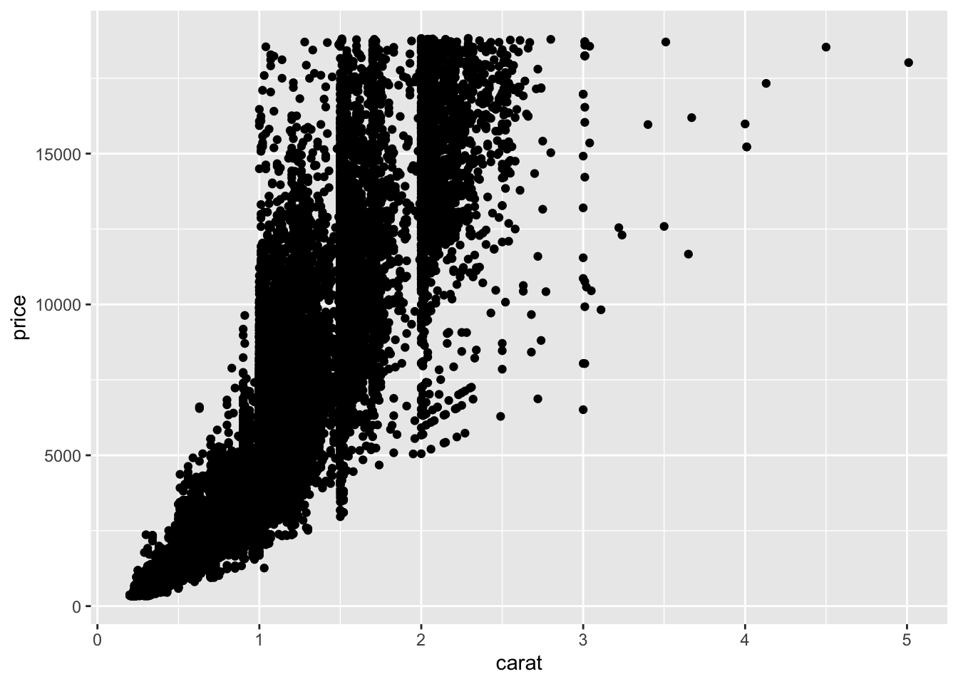
diamonds %>%
  filter(!is.na(price)) %>%
  ggplot(aes(color, price)) +
  geom_boxplot() +
  geom_point(stat="summary", fun=mean, color="red")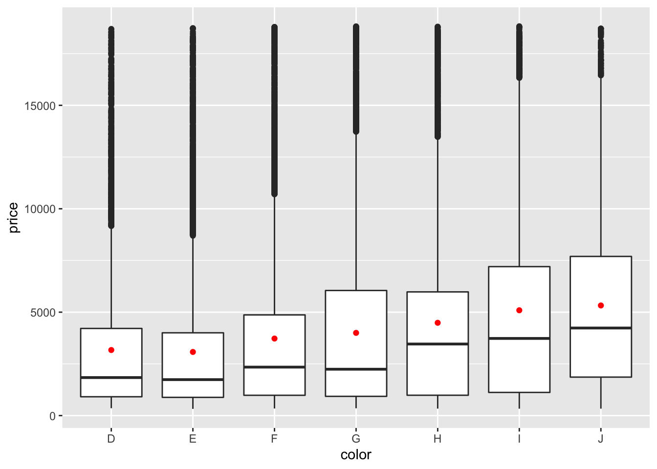
7.3.1 die Regression!
# Zusammenhang Preis Carat
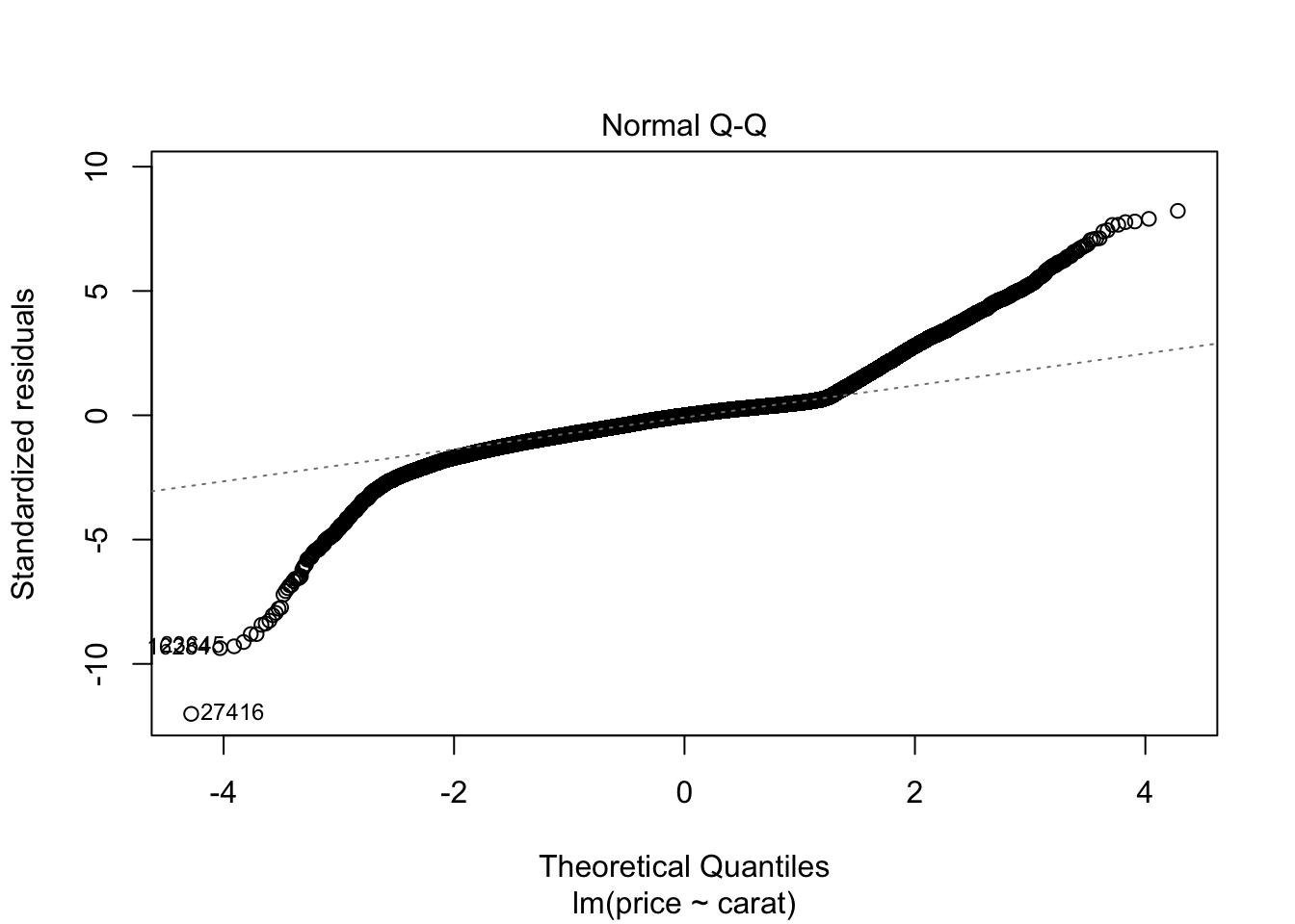
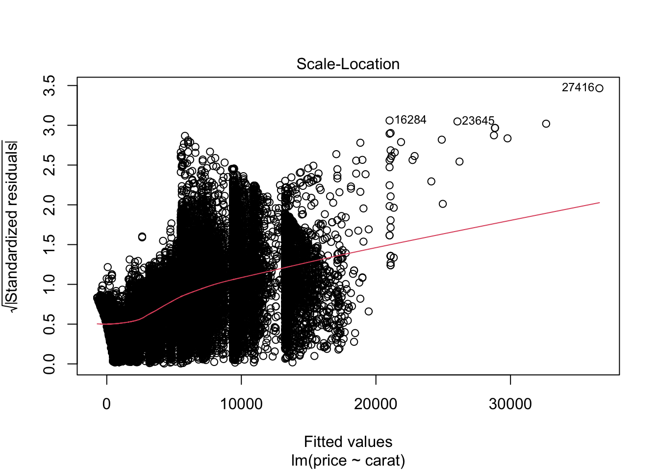
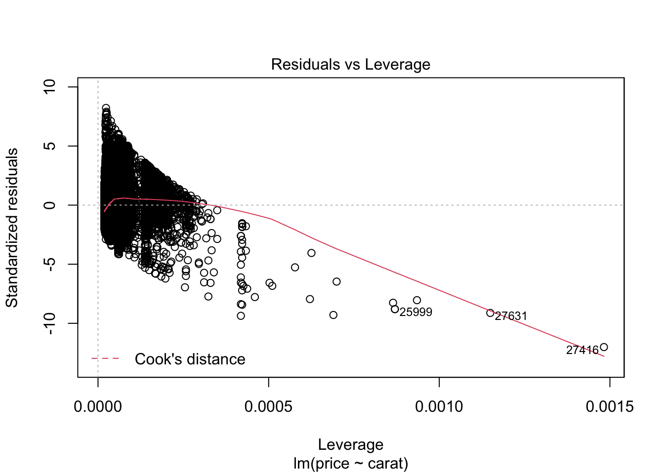
m0 <- lm(price ~ carat, data = diamonds)
summary(m0)##
## Call:
## lm(formula = price ~ carat, data = diamonds)
##
## Residuals:
## Min 1Q Median 3Q Max
## -18585.3 -804.8 -18.9 537.4 12731.7
##
## Coefficients:
## Estimate Std. Error t value Pr(>|t|)
## (Intercept) -2256.36 13.06 -172.8 <2e-16 ***
## carat 7756.43 14.07 551.4 <2e-16 ***
## ---
## Signif. codes:
## 0 '***' 0.001 '**' 0.01 '*' 0.05 '.' 0.1 ' ' 1
##
## Residual standard error: 1549 on 53938 degrees of freedom
## Multiple R-squared: 0.8493, Adjusted R-squared: 0.8493
## F-statistic: 3.041e+05 on 1 and 53938 DF, p-value: < 2.2e-16plot(m0)
m1 <- lm(log(price) ~carat, data = diamonds)
summary(m1)
##
## Call:
## lm(formula = log(price) ~ carat, data = diamonds)
##
## Residuals:
## Min 1Q Median 3Q Max
## -6.2844 -0.2449 0.0335 0.2578 1.5642
##
## Coefficients:
## Estimate Std. Error t value Pr(>|t|)
## (Intercept) 6.215021 0.003348 1856 <2e-16 ***
## carat 1.969757 0.003608 546 <2e-16 ***
## ---
## Signif. codes:
## 0 '***' 0.001 '**' 0.01 '*' 0.05 '.' 0.1 ' ' 1
##
## Residual standard error: 0.3972 on 53938 degrees of freedom
## Multiple R-squared: 0.8468, Adjusted R-squared: 0.8468
## F-statistic: 2.981e+05 on 1 and 53938 DF, p-value: < 2.2e-16#lineares modell mit polynomen
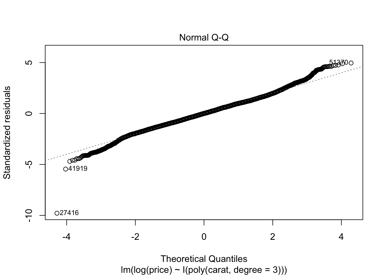
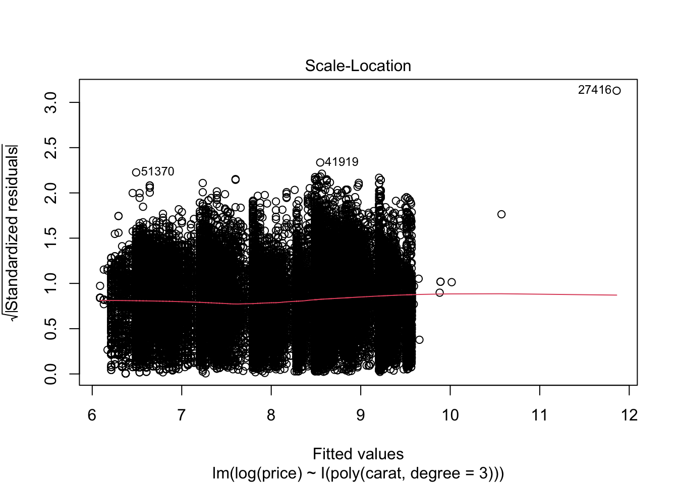
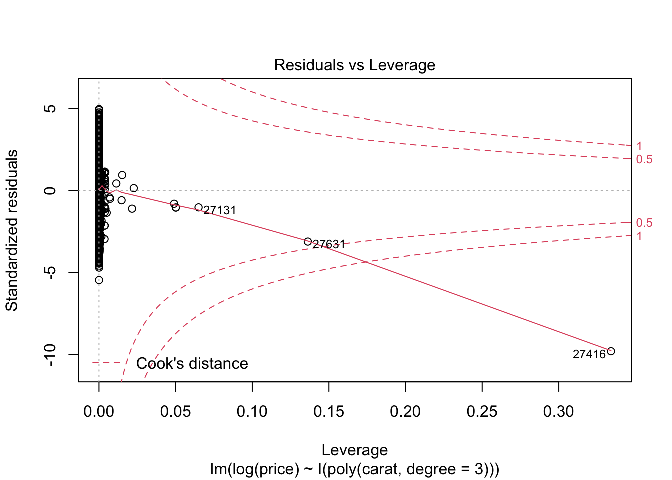
m2 <- lm(log(price) ~ I(poly(carat, degree = 3)), data = diamonds)
summary(m2)##
## Call:
## lm(formula = log(price) ~ I(poly(carat, degree = 3)), data = diamonds)
##
## Residuals:
## Min 1Q Median 3Q Max
## -2.06032 -0.17452 0.00001 0.17349 1.27814
##
## Coefficients:
## Estimate Std. Error
## (Intercept) 7.78677 0.00111
## I(poly(carat, degree = 3))1 216.84668 0.25786
## I(poly(carat, degree = 3))2 -67.76529 0.25786
## I(poly(carat, degree = 3))3 18.16637 0.25786
## t value Pr(>|t|)
## (Intercept) 7013.42 <2e-16 ***
## I(poly(carat, degree = 3))1 840.95 <2e-16 ***
## I(poly(carat, degree = 3))2 -262.80 <2e-16 ***
## I(poly(carat, degree = 3))3 70.45 <2e-16 ***
## ---
## Signif. codes:
## 0 '***' 0.001 '**' 0.01 '*' 0.05 '.' 0.1 ' ' 1
##
## Residual standard error: 0.2579 on 53936 degrees of freedom
## Multiple R-squared: 0.9354, Adjusted R-squared: 0.9354
## F-statistic: 2.604e+05 on 3 and 53936 DF, p-value: < 2.2e-16plot(m2)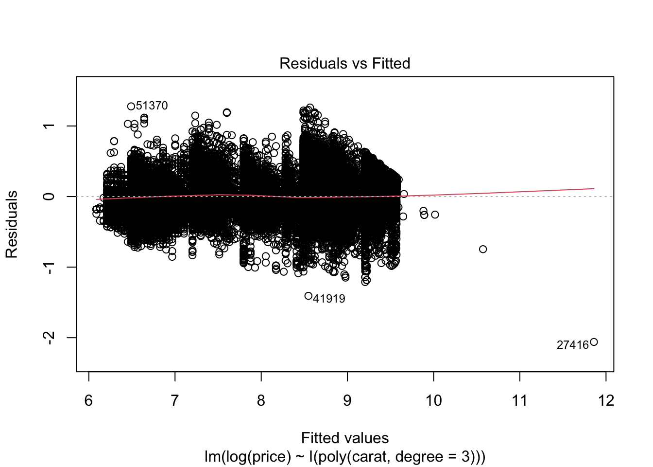
7.4 Aufgabenblatt
library(tidyverse)
swiss <- swiss

# a)
summary(swiss)
## Fertility Agriculture Examination
## Min. :35.00 Min. : 1.20 Min. : 3.00
## 1st Qu.:64.70 1st Qu.:35.90 1st Qu.:12.00
## Median :70.40 Median :54.10 Median :16.00
## Mean :70.14 Mean :50.66 Mean :16.49
## 3rd Qu.:78.45 3rd Qu.:67.65 3rd Qu.:22.00
## Max. :92.50 Max. :89.70 Max. :37.00
## Education Catholic Infant.Mortality
## Min. : 1.00 Min. : 2.150 Min. :10.80
## 1st Qu.: 6.00 1st Qu.: 5.195 1st Qu.:18.15
## Median : 8.00 Median : 15.140 Median :20.00
## Mean :10.98 Mean : 41.144 Mean :19.94
## 3rd Qu.:12.00 3rd Qu.: 93.125 3rd Qu.:21.70
## Max. :53.00 Max. :100.000 Max. :26.60# b)
# Streuung
ggplot(stack(swiss), aes(ind, values)) +
geom_boxplot() +
geom_point(stat="summary", fun="mean", color= "red")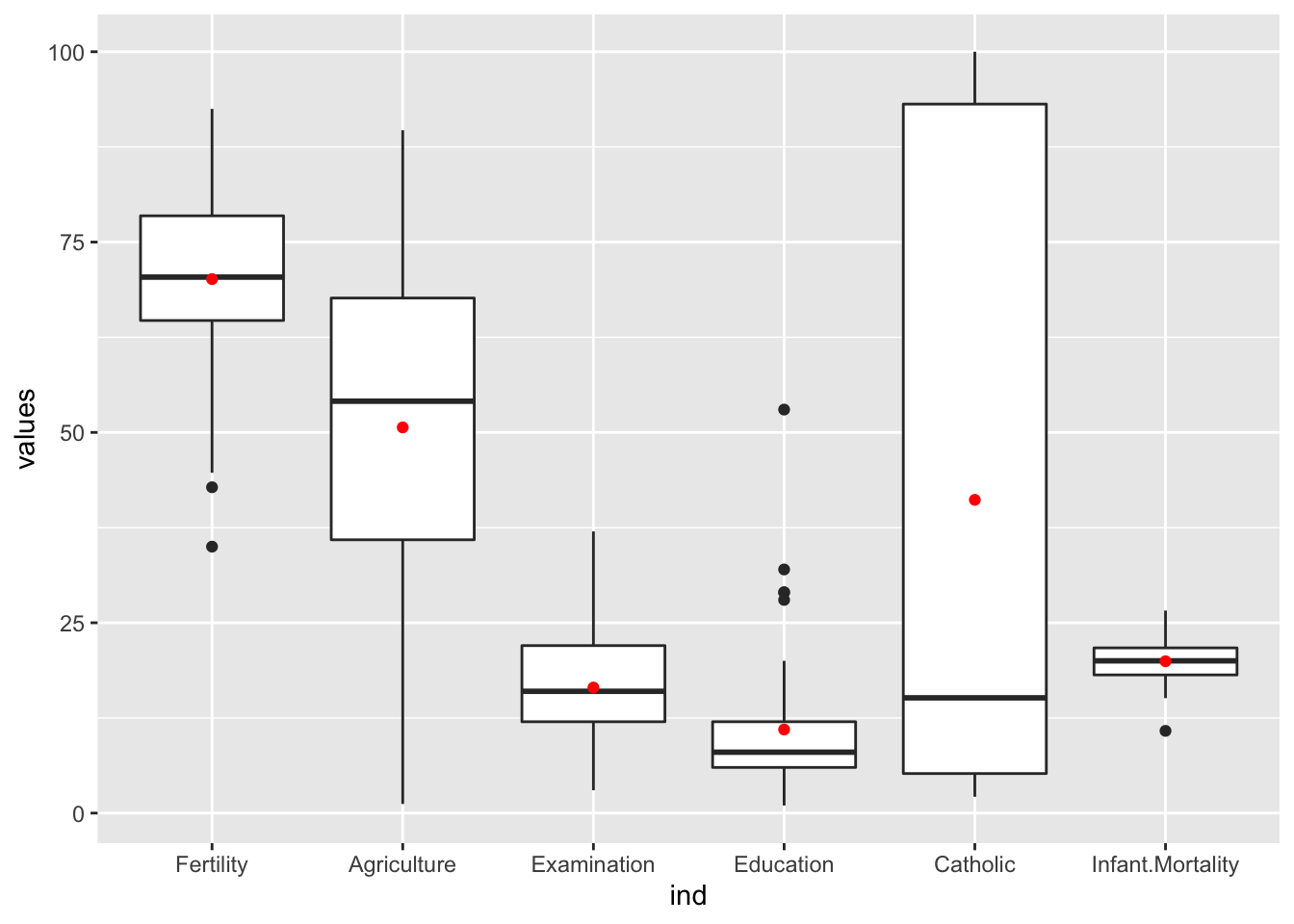
library(GGally)

ggpairs(swiss)
## plot: [1,1] [>-------------------------] 3% est: 0s
## plot: [1,2] [>-------------------------] 6% est: 1s
## plot: [1,3] [=>------------------------] 8% est: 1s
## plot: [1,4] [==>-----------------------] 11% est: 1s
## plot: [1,5] [===>----------------------] 14% est: 1s
## plot: [1,6] [===>----------------------] 17% est: 1s
## plot: [2,1] [====>---------------------] 19% est: 1s
## plot: [2,2] [=====>--------------------] 22% est: 1s
## plot: [2,3] [=====>--------------------] 25% est: 1s
## plot: [2,4] [======>-------------------] 28% est: 1s
## plot: [2,5] [=======>------------------] 31% est: 1s
## plot: [2,6] [========>-----------------] 33% est: 1s
## plot: [3,1] [========>-----------------] 36% est: 1s
## plot: [3,2] [=========>----------------] 39% est: 1s
## plot: [3,3] [==========>---------------] 42% est: 1s
## plot: [3,4] [===========>--------------] 44% est: 1s
## plot: [3,5] [===========>--------------] 47% est: 1s
## plot: [3,6] [============>-------------] 50% est: 1s
## plot: [4,1] [=============>------------] 53% est: 1s
## plot: [4,2] [=============>------------] 56% est: 1s
## plot: [4,3] [==============>-----------] 58% est: 1s
## plot: [4,4] [===============>----------] 61% est: 1s
## plot: [4,5] [================>---------] 64% est: 0s
## plot: [4,6] [================>---------] 67% est: 0s
## plot: [5,1] [=================>--------] 69% est: 0s
## plot: [5,2] [==================>-------] 72% est: 0s
## plot: [5,3] [===================>------] 75% est: 0s
## plot: [5,4] [===================>------] 78% est: 0s
## plot: [5,5] [====================>-----] 81% est: 0s
## plot: [5,6] [=====================>----] 83% est: 0s
## plot: [6,1] [=====================>----] 86% est: 0s
## plot: [6,2] [======================>---] 89% est: 0s
## plot: [6,3] [=======================>--] 92% est: 0s
## plot: [6,4] [========================>-] 94% est: 0s
## plot: [6,5] [========================>-] 97% est: 0s
## plot: [6,6] [==========================]100% est: 0s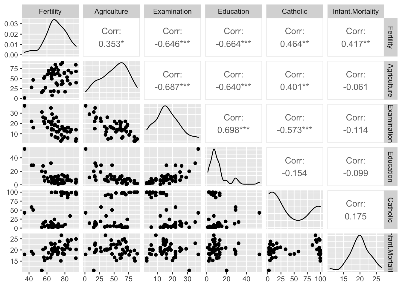
7.5 Lineares Modell
benötigt: passende Variablen Methodne zur Variablenselektion hier S. 96
Vorwärtsverfahren: - Variable mit höchster Korrelation auswählen und R^2 testen - immer weiter Variablen hinzufügen und R^2 testen - solange R^2 Veränderung signifikant ist : weitermachen
# education
model <- lm(Fertility ~ Education, data= swiss)
summary(model)$r.squared
## [1] 0.4406156# R^2 = 0.44R^2 hier nur 44% (44% der Variation kann dadurch erklärt werden)
-> multi lineares Modell testen mit weiteren Variabln
# weitere Variable Catholic
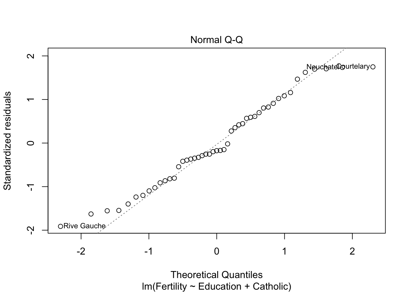
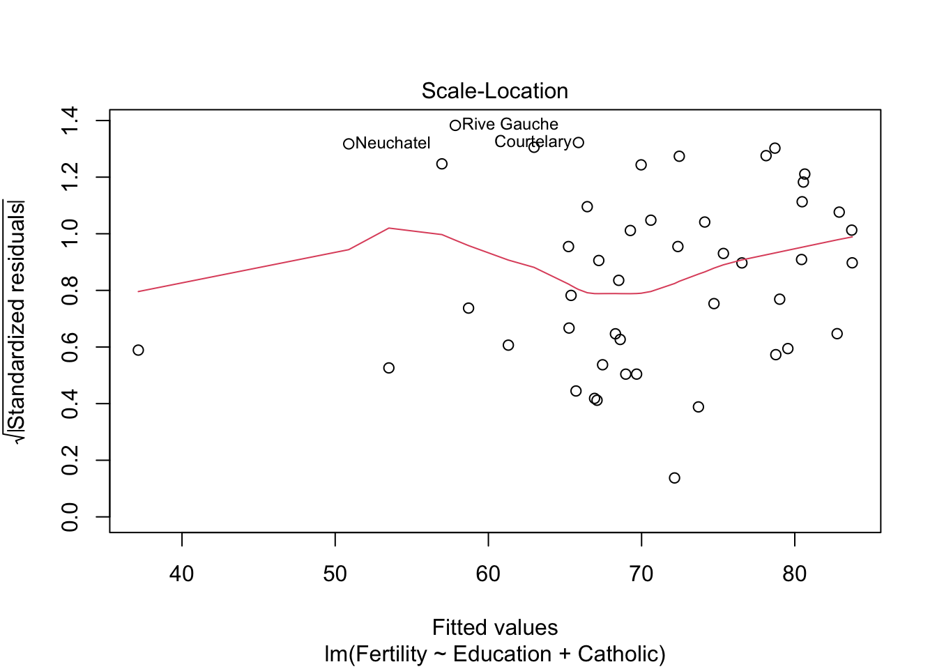
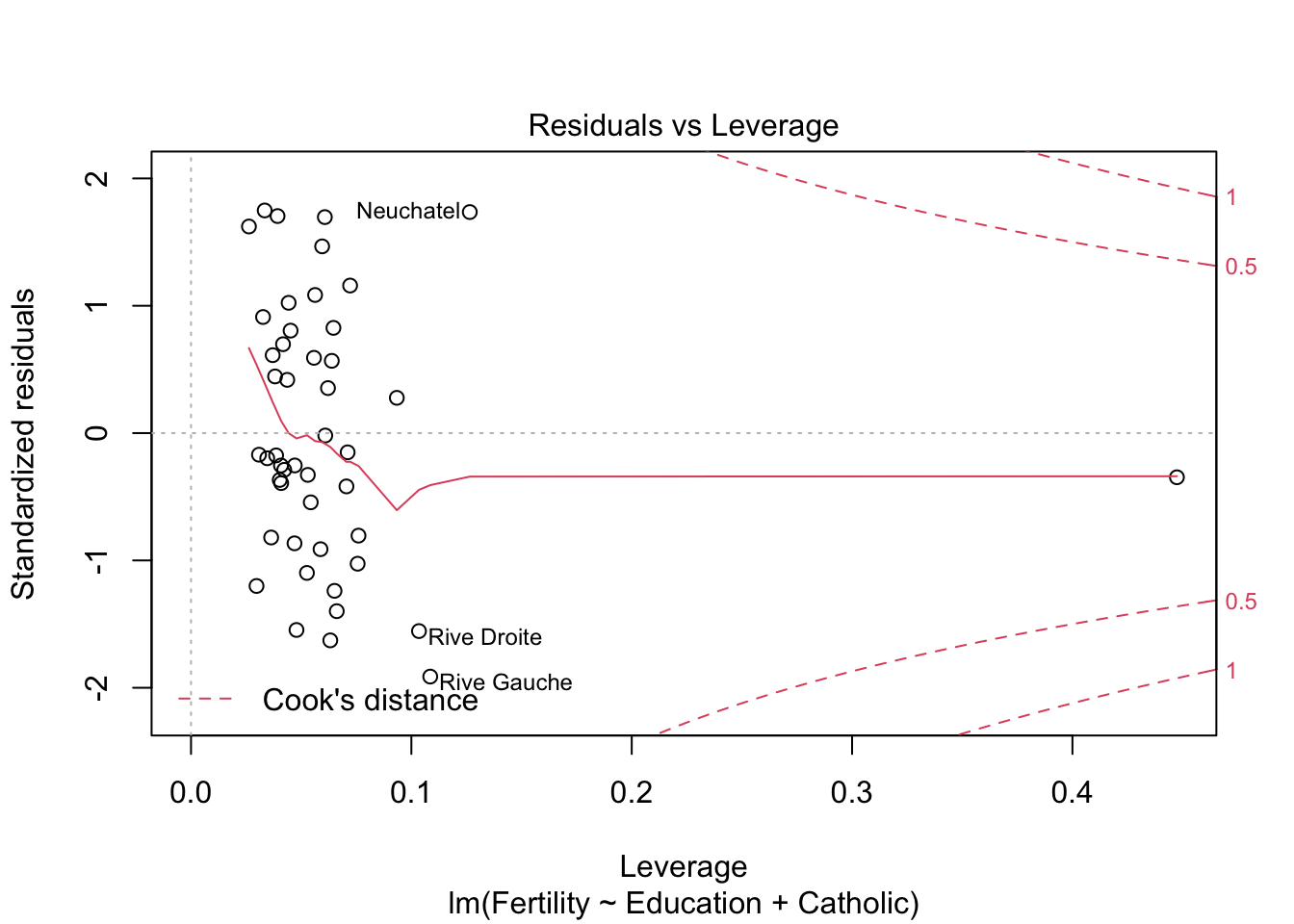
model2 <- lm(Fertility ~ Education+Catholic, data= swiss)
summary(model2)$r.squared## [1] 0.5745071# R^2 => 0.57
# delta R^2 = 0.11 (gut!)
# Agriculture
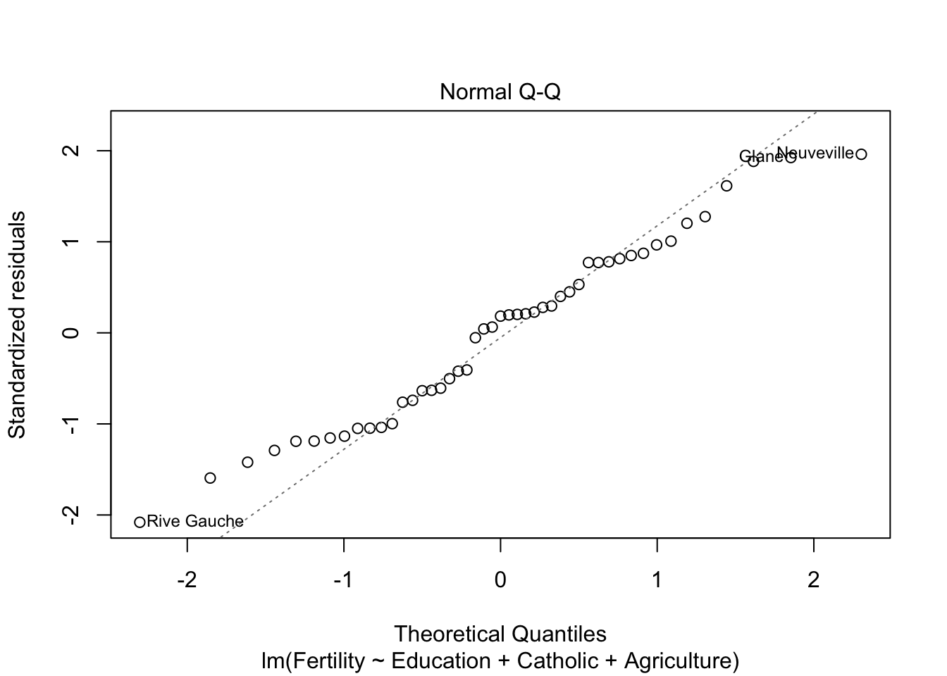
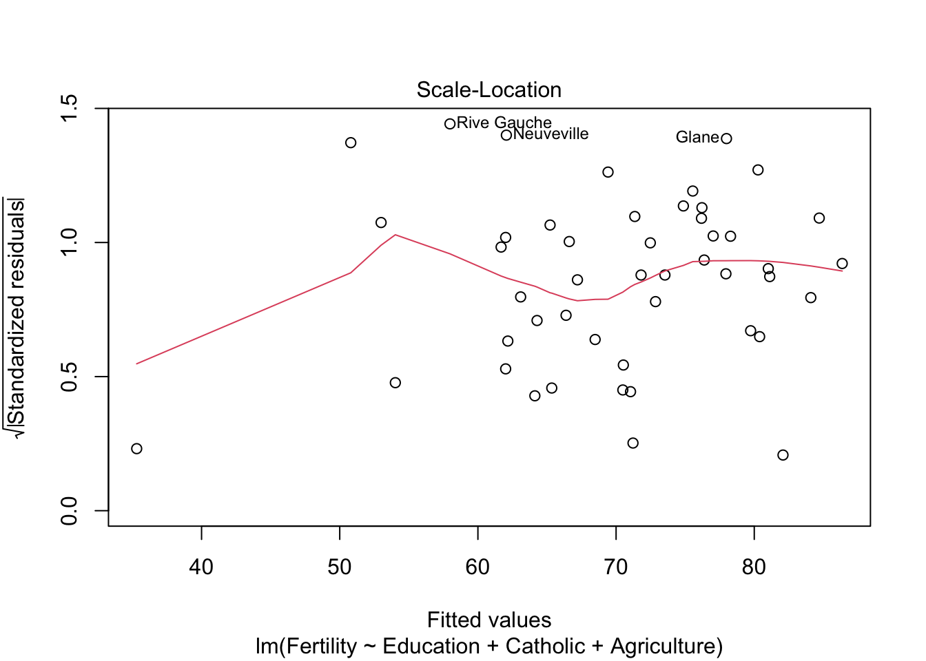
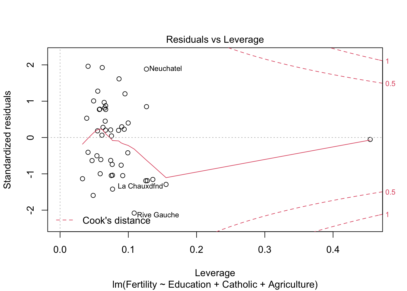
model3 <- lm(Fertility ~ Education+Catholic+Agriculture, data= swiss)
summary(model3)$r.squared## [1] 0.6422541# R^2 = 0.64
# delta R^2 = 0,07 (auch gut!)
model4 <- lm(Fertility ~ Education+Catholic+Agriculture+Examination, data= swiss)
summary(model4)$r.squared## [1] 0.6497897# r^2 ändert sich fast nichtalso Model3 oder model2
plot(model2) #besser bei panel 2+4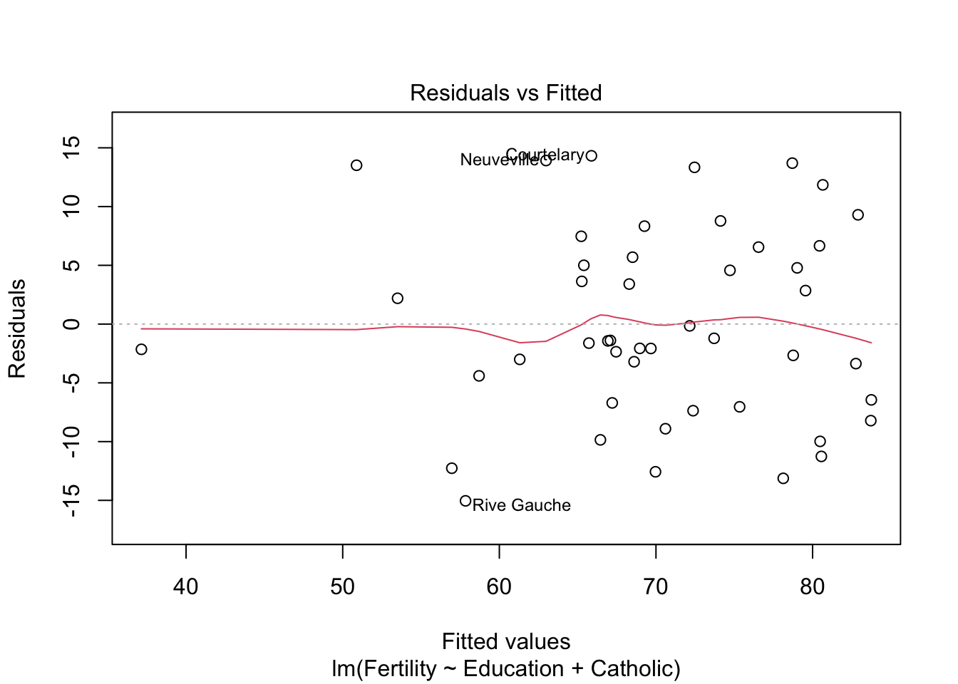
plot(model3)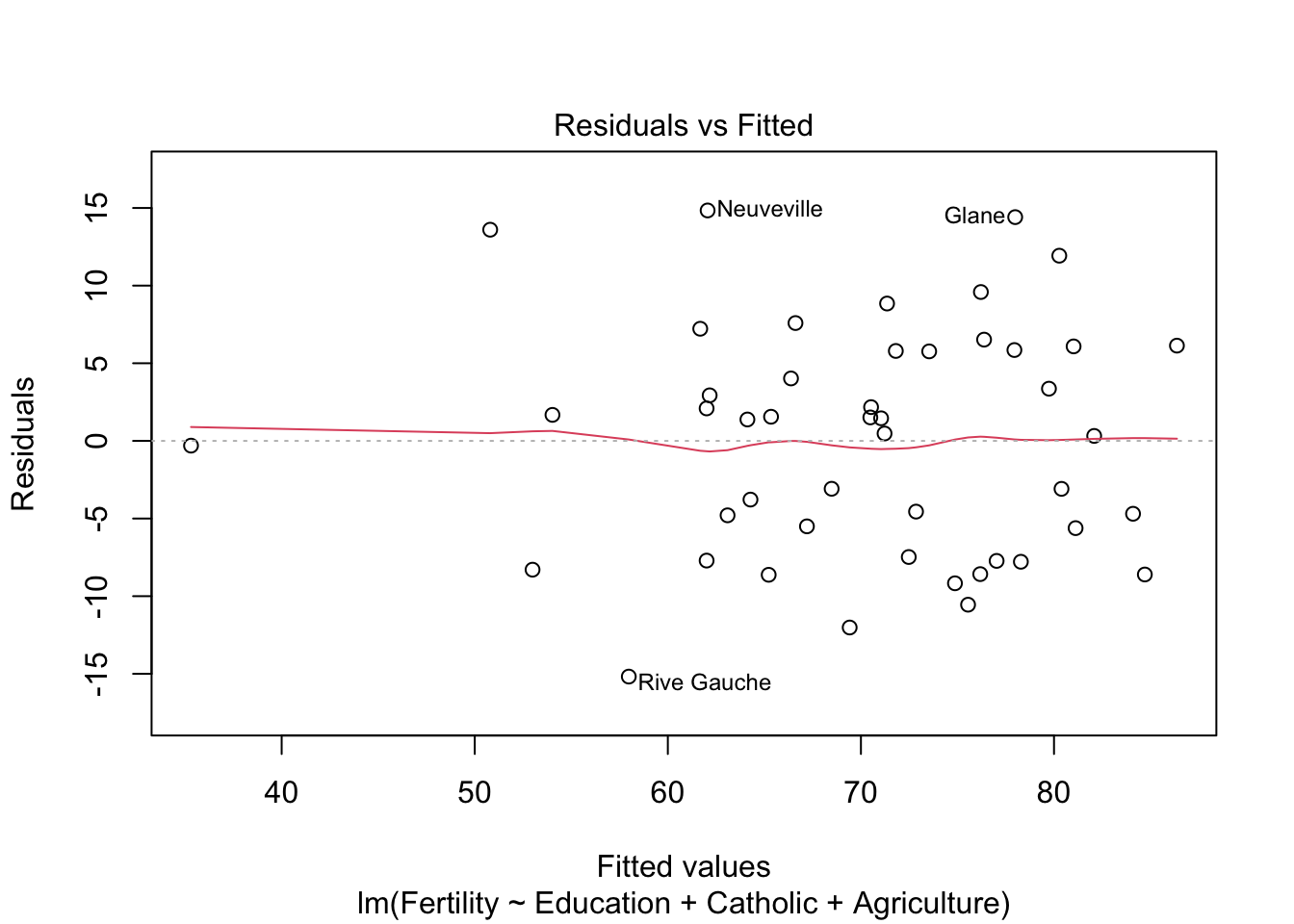
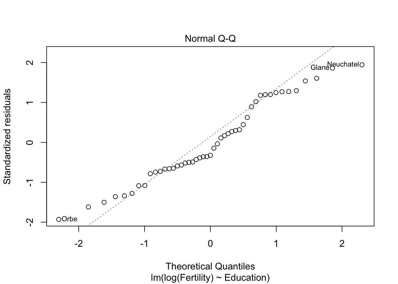
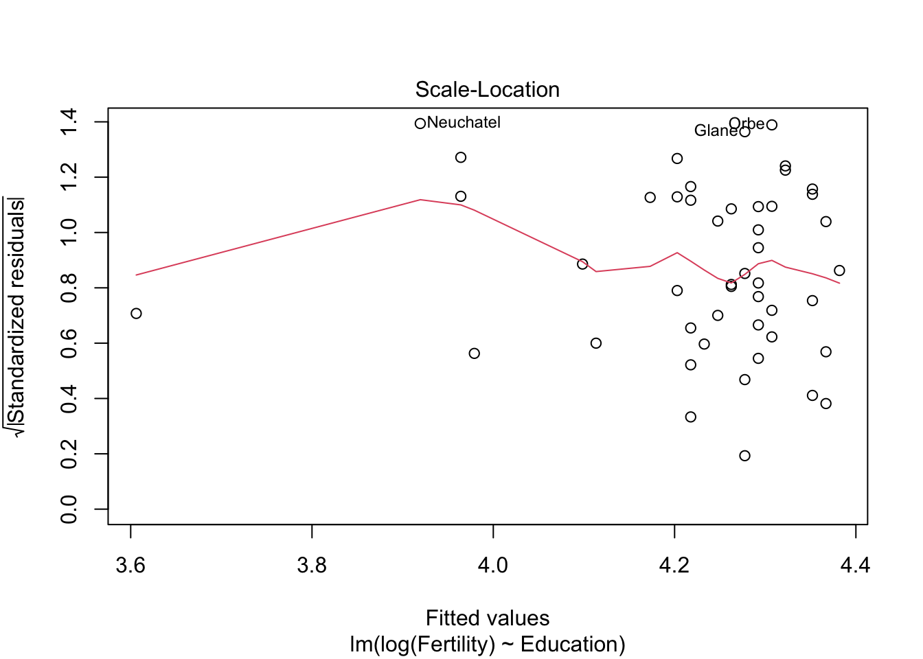
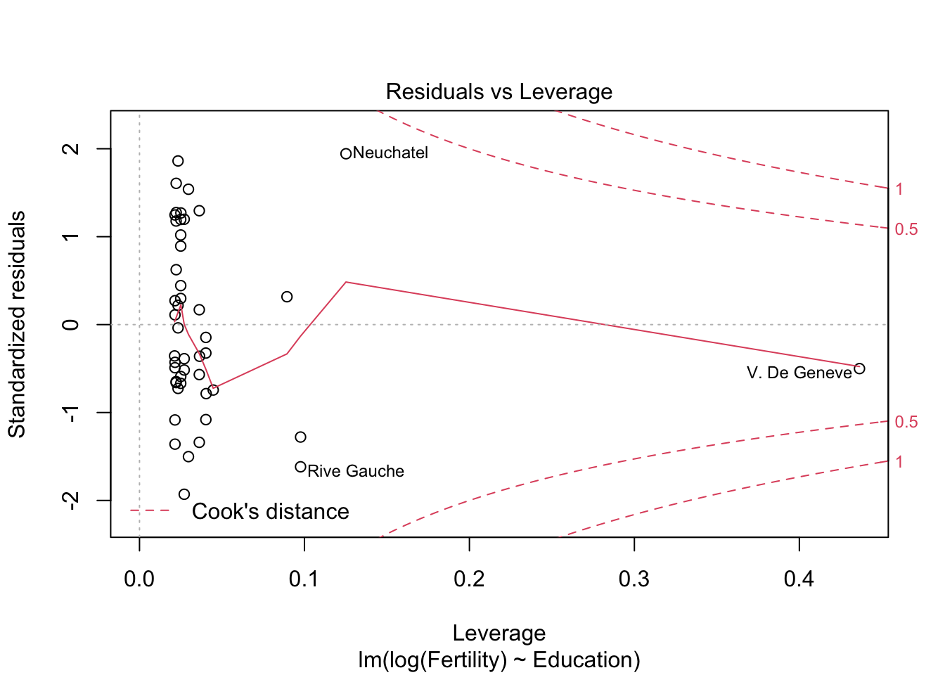
m1 <- lm(log(Fertility) ~ Education, data= swiss)
summary(m1)
##
## Call:
## lm(formula = log(Fertility) ~ Education, data = swiss)
##
## Residuals:
## Min 1Q Median 3Q Max
## -0.25727 -0.08868 -0.04285 0.12762 0.24865
##
## Coefficients:
## Estimate Std. Error t value Pr(>|t|)
## (Intercept) 4.396825 0.030110 146.024 < 2e-16 ***
## Education -0.014919 0.002073 -7.198 5.2e-09 ***
## ---
## Signif. codes:
## 0 '***' 0.001 '**' 0.01 '*' 0.05 '.' 0.1 ' ' 1
##
## Residual standard error: 0.1352 on 45 degrees of freedom
## Multiple R-squared: 0.5351, Adjusted R-squared: 0.5248
## F-statistic: 51.8 on 1 and 45 DF, p-value: 5.195e-09# r^2 0.57 > 0.44
plot(m1)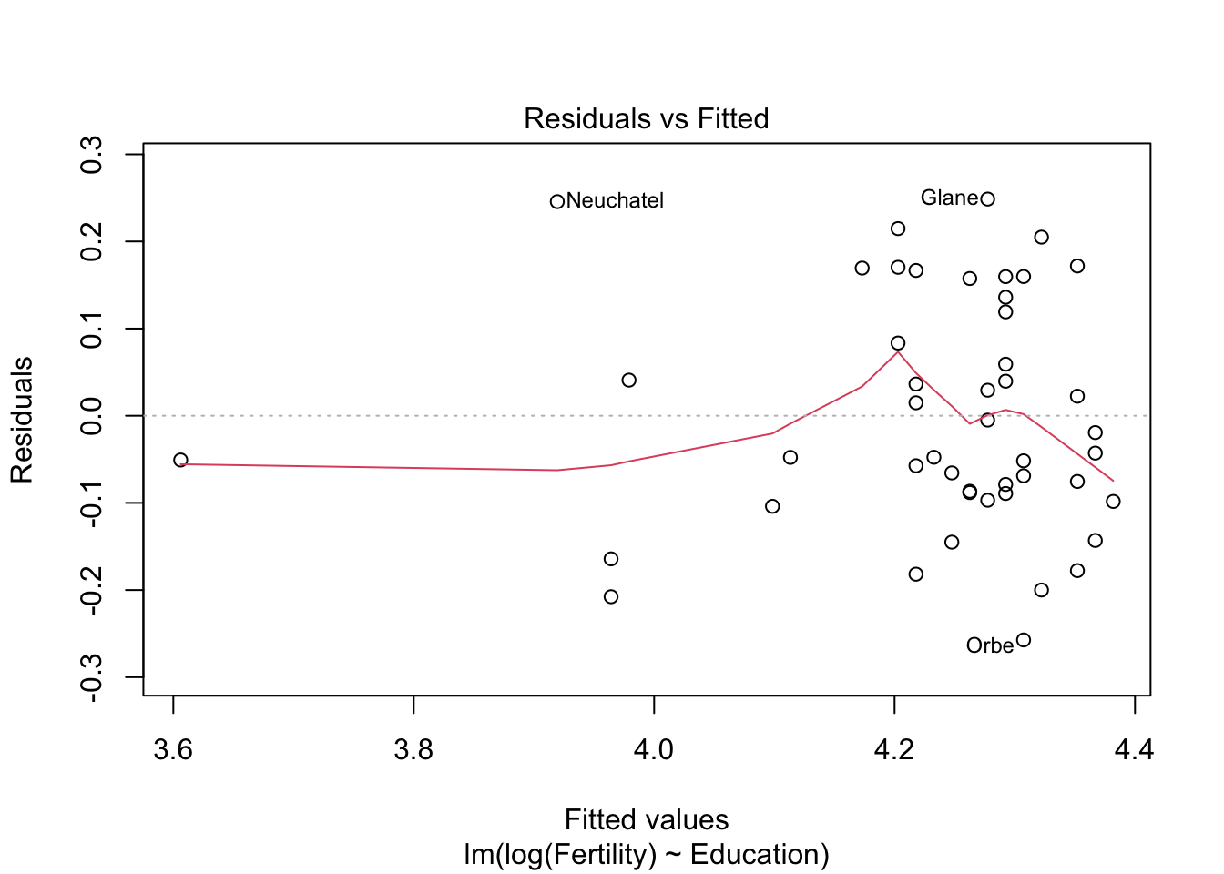
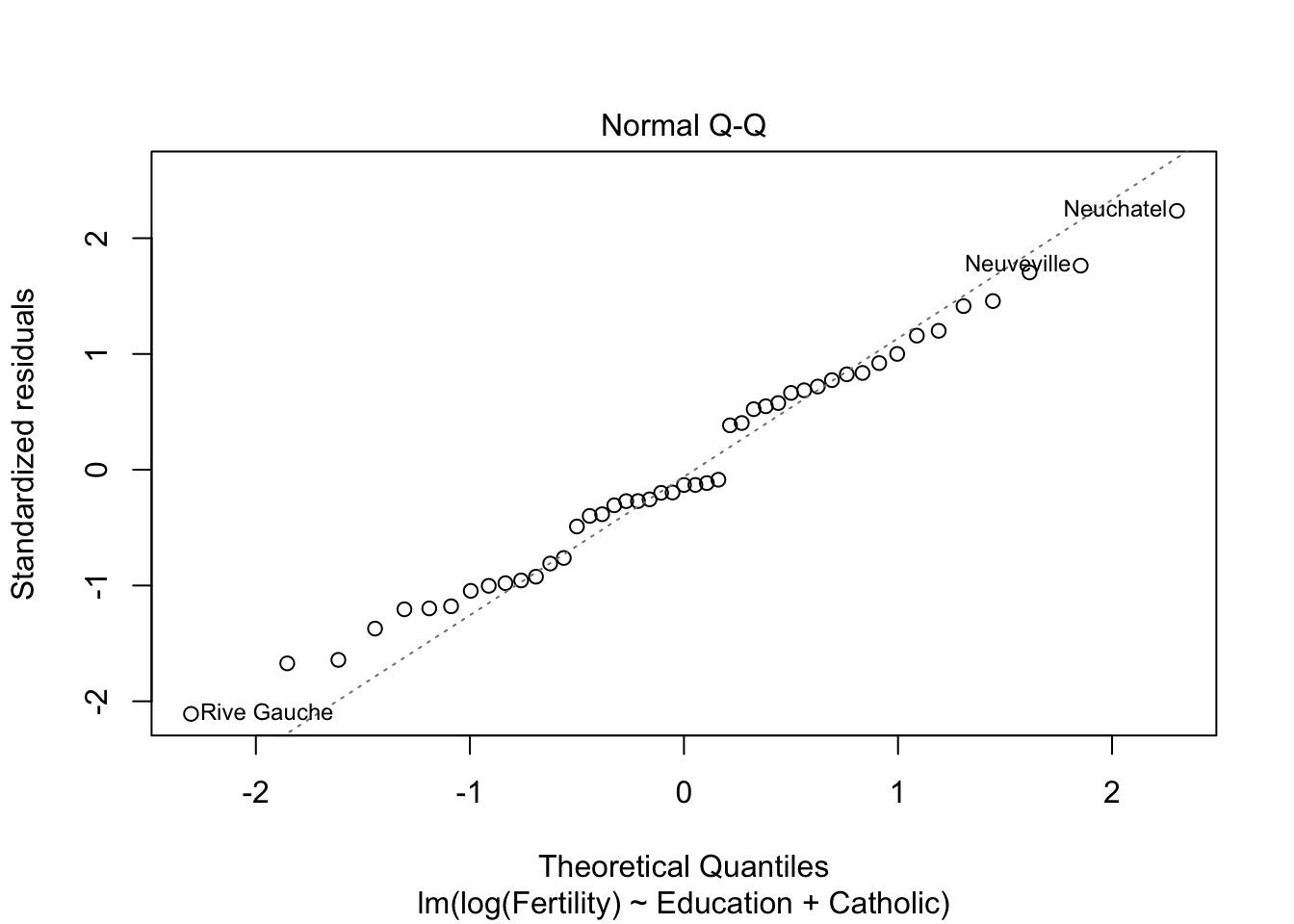
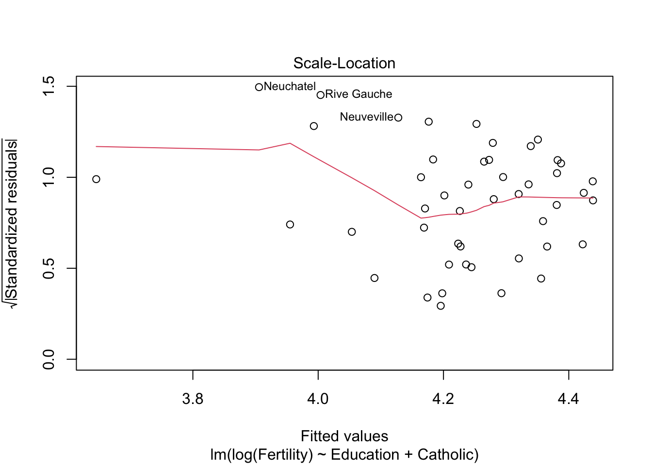
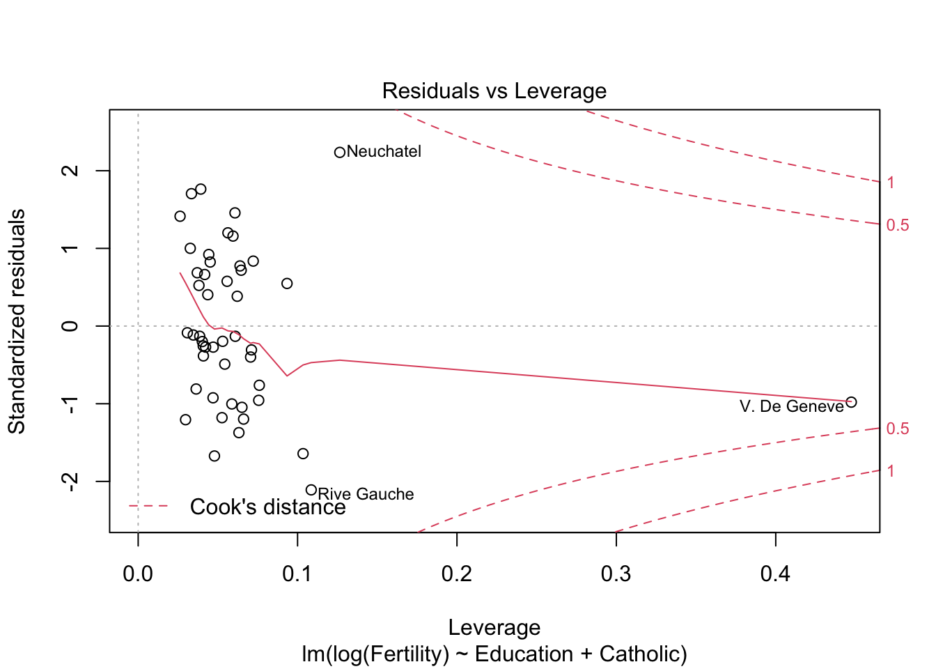
m2 <- lm(log(Fertility) ~ Education+Catholic, data= swiss)
summary(m2)$r.squared #r^2 = 0.61 > 0.57
## [1] 0.6163616plot(m2)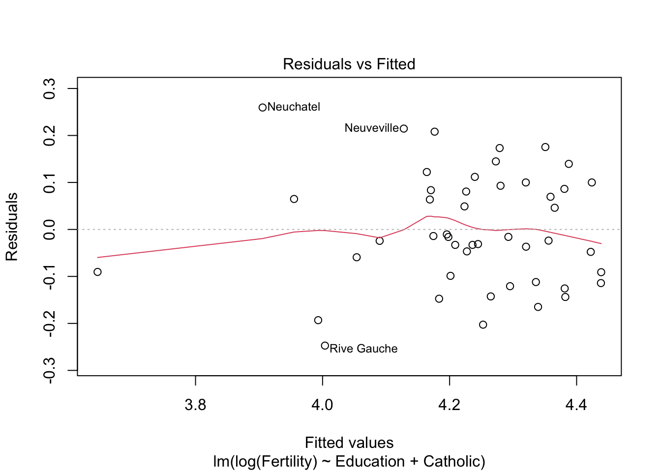
m3 <- lm(Fertility ~ Education+Catholic+Agriculture, data= swiss)
summary(m3)$r.squared
## [1] 0.6422541library(robustbase)
model_robust <- lmrob(log(Fertility) ~ Education, data= swiss)
summary(model_robust)##
## Call:
## lmrob(formula = log(Fertility) ~ Education, data = swiss)
## \--> method = "MM"
## Residuals:
## Min 1Q Median 3Q Max
## -0.25564 -0.08674 -0.04180 0.12940 0.25139
##
## Coefficients:
## Estimate Std. Error t value Pr(>|t|)
## (Intercept) 4.396133 0.029191 150.60 < 2e-16 ***
## Education -0.015075 0.002013 -7.49 1.92e-09 ***
## ---
## Signif. codes:
## 0 '***' 0.001 '**' 0.01 '*' 0.05 '.' 0.1 ' ' 1
##
## Robust residual standard error: 0.1471
## Multiple R-squared: 0.5152, Adjusted R-squared: 0.5044
## Convergence in 7 IRWLS iterations
##
## Robustness weights:
## one weight is ~= 1. The remaining 46 ones are summarized as
## Min. 1st Qu. Median Mean 3rd Qu. Max.
## 0.7438 0.8798 0.9614 0.9276 0.9890 0.9987
## Algorithmic parameters:
## tuning.chi bb tuning.psi
## 1.548e+00 5.000e-01 4.685e+00
## refine.tol rel.tol scale.tol
## 1.000e-07 1.000e-07 1.000e-10
## solve.tol eps.outlier eps.x
## 1.000e-07 2.128e-03 9.641e-11
## warn.limit.reject warn.limit.meanrw
## 5.000e-01 5.000e-01
## nResample max.it best.r.s
## 500 50 2
## k.fast.s k.max maxit.scale
## 1 200 200
## trace.lev mts compute.rd
## 0 1000 0
## fast.s.large.n
## 2000
## psi subsampling
## "bisquare" "nonsingular"
## cov compute.outlier.stats
## ".vcov.avar1" "SM"
## seed : int(0)#R^2 = 0.51 > 0.57 von davorBerechnung (aus lmrob) : MM-type Methode im Gegensatz zur least-squares Methode
verbessert R^2 Ergebnis aber nicht, und Rest kann ich nicht bewerten