Empirical Economics with R

Intro

Dependent Variable = intercept + ß explanatory variable + error

\[ y = \alpha + \beta x + \mu \]

\(\beta\) estimated with Ordinary Least Squares (OLS)
explanatory variable = should be exogenous

Acemoglus Regression

Formula

\[ \log y_i = \mu + aR_i+\bf{X}_i \gamma+ \epsilon \]

Figure:

Table:

empty lines = not included in regression
- every new sample = broader regression formula with dummies etc.
\(R^2 = 0.62\): goodness of fit of regression line
- quite good here (explains 62% of the variance)
Sample 7/8 new dependent variable to make it more solid

Interlude: Regression Interpretation

Modell	Abhängige Var.	Erklärende Var.	Interpretation
Level-Level	y	\(x_j\)	\(\Delta \hat{y} = \beta_j \Delta x_j\)
Level-Log	y	\(log(x_j)\)	\(\Delta \hat{y} = \frac{\beta_j}{100} \% \Delta x_j\)
Log-Level	log(y)	\(x_j\)	\(\% \Delta \hat{y} = 100 \beta_j \Delta x_j\)
Log-Log	log(y)	log(x)	\(\% \Delta \hat{y} = \beta_j \% \Delta x_j\)

=> ours is log-level

Recreation of the Table

library(stargazer)

Warning: Paket 'stargazer' wurde unter R Version 4.1.2 erstellt


Please cite as:

 Hlavac, Marek (2022). stargazer: Well-Formatted Regression and Summary Statistics Tables.

 R package version 5.2.3. https://CRAN.R-project.org/package=stargazer

load("data/dataset_AJR2001.Rdata")
head(data)

Table 2: Estimation of Models 1-4 for both datasets

Table Column Names:

logpgp95= Log GDP per capita, PPP, 1995
avexpr = Average protection against expropriation risk, 1985-1995
baseco = Dummy variable for countries in the base sample (colonized)
lat_abst = Absolute value of latitude
loghjypl = Log output per worker in 1988 (US normalized to 1)

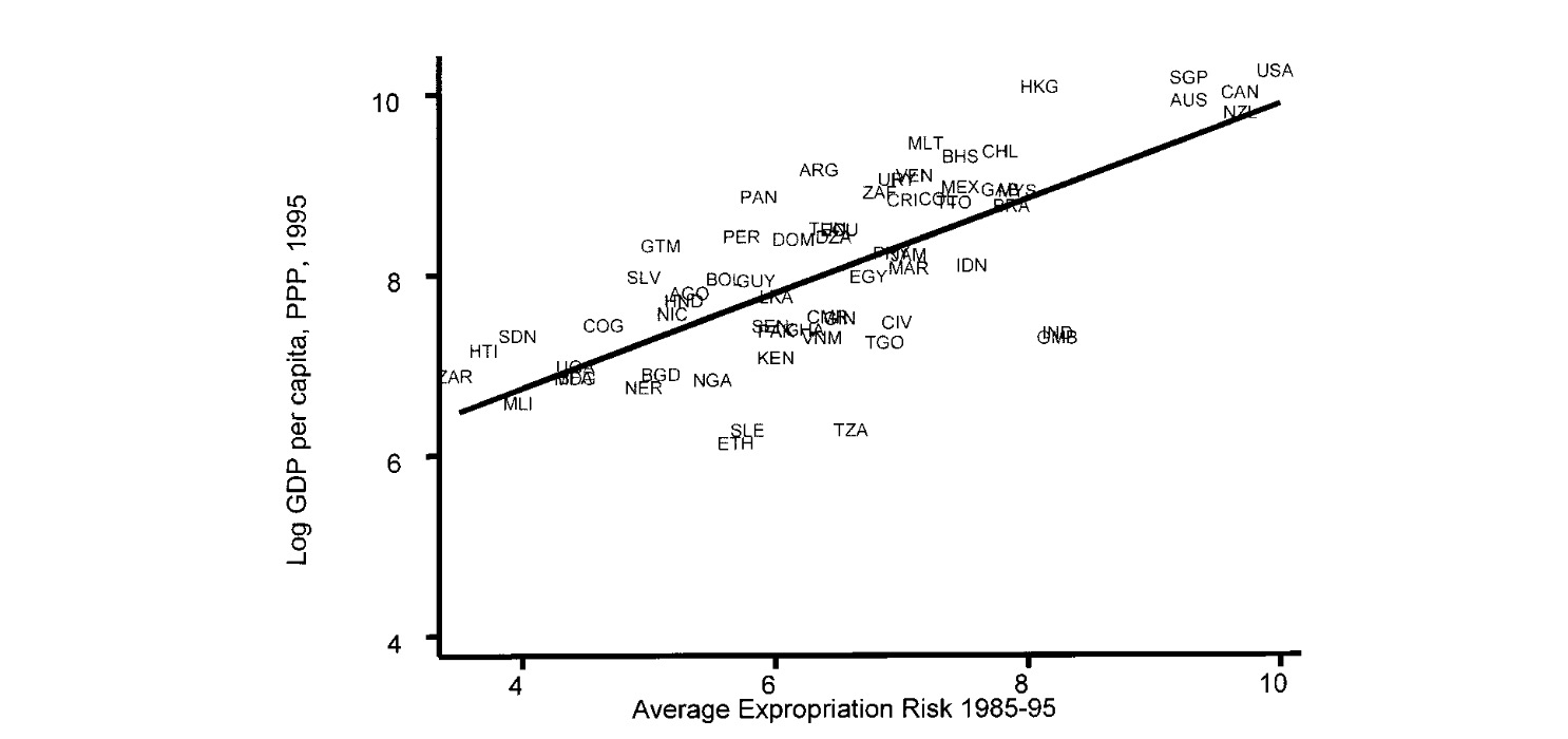
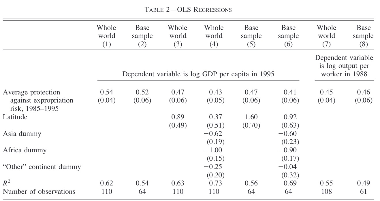
m_T2_world_1 <- lm(logpgp95 ~ avexpr, data=data)
m_T2_base_1 <- lm(logpgp95 ~ avexpr, data=data[which(data$baseco==1),])

#latitude added
m_T2_world_2 <- lm(logpgp95 ~avexpr + lat_abst,data=data)
m_T2_base_2 <- lm(logpgp95 ~ avexpr + lat_abst, data=data[which(data$baseco==1),])

# continent dummies
m_T2_world_3 <- lm(logpgp95 ~avexpr + lat_abst + asia + africa + other,data=data)
m_T2_base_3 <- lm(logpgp95 ~ avexpr + lat_abst + asia + africa + other, data=data[which(data$baseco==1),])

# other dependent variable
m_T2_world_4 <- lm(loghjypl ~avexpr, data=data)
m_T2_base_4 <- lm(loghjypl ~ avexpr, data=data[which(data$baseco==1),])

Summary of the first Regression

summary(m_T2_world_1)


Call:
lm(formula = logpgp95 ~ avexpr, data = data)

Residuals:
    Min      1Q  Median      3Q     Max 
-1.9020 -0.3160  0.1380  0.4225  1.4406 

Coefficients:
            Estimate Std. Error t value Pr(>|t|)    
(Intercept)  4.62609    0.30058   15.39   <2e-16 ***
avexpr       0.53187    0.04062   13.09   <2e-16 ***
---
Signif. codes:  0 '***' 0.001 '**' 0.01 '*' 0.05 '.' 0.1 ' ' 1

Residual standard error: 0.7179 on 109 degrees of freedom
  (52 Beobachtungen als fehlend gelöscht)
Multiple R-squared:  0.6113,    Adjusted R-squared:  0.6078 
F-statistic: 171.4 on 1 and 109 DF,  p-value: < 2.2e-16

Now we have the Regression Models, but until now no Table to present these

all_res <- list(
  m_T2_world_1, m_T2_base_1,
  m_T2_world_2, m_T2_base_2,
  m_T2_world_3, m_T2_base_3,
  m_T2_world_4, m_T2_base_4
  )
coef_names <- c("Average Protection", "Latittude","Asia dummy", "Africa dummy", "Other")
note <- "Nitzuen lorem"
stargazer(all_res, 
          type="html", 
          out="data/Table2_stargazer.html", omit = "Constant",
          notes.label = note,
          dep.var.labels = c("log GDP per Capita", "log output per worker"),
          covariate.labels = coef_names
          )


	Dependent variable:

	log GDP per Capita						log output per worker
	(1)	(2)	(3)	(4)	(5)	(6)	(7)	(8)

Average Protection	0.532^***	0.522^***	0.463^***	0.468^***	0.390^***	0.401^***	0.446^***	0.457^***
	(0.041)	(0.061)	(0.055)	(0.064)	(0.051)	(0.059)	(0.039)	(0.061)

Latittude			0.872^*	1.577^**	0.333	0.875
			(0.488)	(0.710)	(0.445)	(0.628)

Asia dummy					-0.153	-0.577^**
					(0.155)	(0.231)

Africa dummy					-0.916^***	-0.881^***
					(0.166)	(0.170)

Other					0.304	0.107
					(0.375)	(0.382)


Observations	111	64	111	64	111	64	108	61
R²	0.611	0.540	0.623	0.574	0.715	0.714	0.554	0.486
Adjusted R²	0.608	0.533	0.616	0.561	0.702	0.689	0.550	0.477
Residual Std. Error	0.718 (df = 109)	0.713 (df = 62)	0.711 (df = 108)	0.692 (df = 61)	0.626 (df = 105)	0.582 (df = 58)	0.713 (df = 106)	0.709 (df = 59)
F Statistic	171.438^*** (df = 1; 109)	72.816^*** (df = 1; 62)	89.047^*** (df = 2; 108)	41.179^*** (df = 2; 61)	52.738^*** (df = 5; 105)	28.946^*** (df = 5; 58)	131.705^*** (df = 1; 106)	55.828^*** (df = 1; 59)

Nitzuen lorem	p<0.1; p<0.05; p<0.01

26.10.2023 Regression

Intro

Acemoglus Regression

Interlude: Regression Interpretation

Recreation of the Table