Empirical Economics with R

Time Series

library(tseries)

Registered S3 method overwritten by 'quantmod':
  method            from
  as.zoo.data.frame zoo

Import Data

data <- read.table("data/Per_Capita_GDP_Data_1870-1987.asc", header=T)
head(data)

Bind the Column and Data set together = cbind()

startyear <- 1870
year <- seq(from=startyear, to= 1987, by=1)
data_GDP <- cbind(year, data) 
head(data_GDP) # new year column

Define Time Series

data_ts <- ts(data_GDP, startyear)
class(data_ts)

[1] "mts"    "ts"     "matrix"

[1] "mts"    "ts"     "matrix"

MTS = multiple Time Series

apply diff

us_diff <- diff(log(data_ts[,"USA"]))

Take the Column USA
log the GDP
now take the Difference \(\Delta y = y_{t} - y_{t-1}\)

=> Growth Rate of Log GDP in USA

Plot

plot(data_ts[,c("USA")])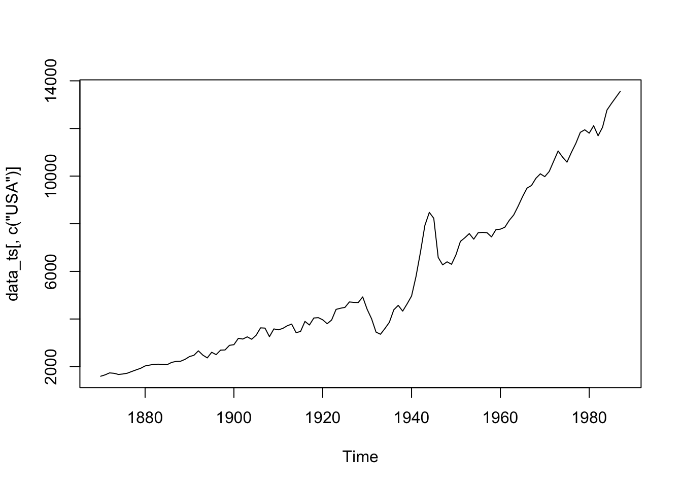

plot(us_diff)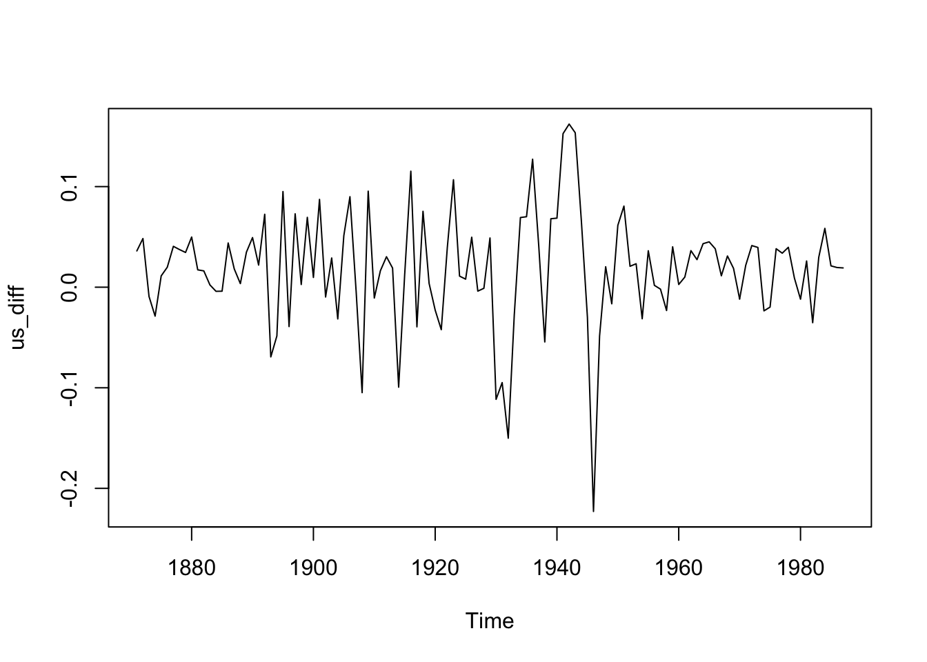

Panel Data

library(plm)

Warning: Paket 'plm' wurde unter R Version 4.1.2 erstellt

library(stargazer)

Warning: Paket 'stargazer' wurde unter R Version 4.1.2 erstellt


Please cite as:

 Hlavac, Marek (2022). stargazer: Well-Formatted Regression and Summary Statistics Tables.

 R package version 5.2.3. https://CRAN.R-project.org/package=stargazer

data(wagepan, package='wooldridge') # directly from package witoout loading
head(wagepan)

Get Panel Data from thsi with pdata.frame()

wagepan.p <- pdata.frame(wagepan, index=c("nr","year") ) #added HA: individual index and time index
pdim(wagepan.p)

Balanced Panel: n = 545, T = 8, N = 4360

n = number of individuals / regions = 545
T = Number of observations of the indiviudals = 8
N = n*T

Regressions with plm()

1) Simple linear Regression with all data pooled

wagemodel1 <- plm(lwage ~ married + union + exper, data=wagepan.p, model="pooling")

2) now same as above but with controls

wagemodel2 <- plm(lwage ~ married + black + union + educ + exper, data=wagepan.p, model="pooling")

3) estimate fixed effects model (based on “within-transformation” of data) <–> pooling model

NOTE: use for my Acemoglu Paper!!

wagemodel3 <- plm(lwage ~ married + union + educ + exper, data=wagepan.p, model="within")

Summary

summary(wagemodel3)

Oneway (individual) effect Within Model

Call:
plm(formula = lwage ~ married + union + educ + exper, data = wagepan.p, 
    model = "within")

Balanced Panel: n = 545, T = 8, N = 4360

Residuals:
    Min.  1st Qu.   Median  3rd Qu.     Max. 
-4.14628 -0.12503  0.01232  0.16205  1.48094 

Coefficients:
         Estimate Std. Error t-value  Pr(>|t|)    
married 0.0610384  0.0182929  3.3367 0.0008558 ***
union   0.0837910  0.0194140  4.3160 1.629e-05 ***
exper   0.0598672  0.0025835 23.1726 < 2.2e-16 ***
---
Signif. codes:  0 '***' 0.001 '**' 0.01 '*' 0.05 '.' 0.1 ' ' 1

Total Sum of Squares:    572.05
Residual Sum of Squares: 476.43
R-Squared:      0.16715
Adj. R-Squared: 0.047646
F-statistic: 255.026 on 3 and 3812 DF, p-value: < 2.22e-16

4) same, but with year dummy for shock absorption

Used with factor(year) for easy year incuding of the variables

wagemodel4 <- plm(lwage ~ married + black + union + educ + exper + factor(year), data=wagepan.p, model="pooling")

Combine all and get stargazer to analyze it

mywagemodels <- list(wagemodel1,wagemodel2,wagemodel3,wagemodel4)
stargazer(
  mywagemodels, 
  type="html"
  #out="data/mywagemodels.html"
  )


	Dependent variable:

	lwage
	(1)	(2)	(3)	(4)

married	0.174^***	0.113^***	0.061^***	0.111^***
	(0.016)	(0.016)	(0.018)	(0.016)

black		-0.145^***		-0.140^***
		(0.023)		(0.023)

union	0.169^***	0.184^***	0.084^***	0.187^***
	(0.018)	(0.017)	(0.019)	(0.017)

educ		0.103^***		0.092^***
		(0.004)		(0.005)

exper	0.025^***	0.050^***	0.060^***	0.030^***
	(0.003)	(0.003)	(0.003)	(0.005)

factor(year)1981				0.078^***
				(0.030)

factor(year)1982				0.097^***
				(0.031)

factor(year)1983				0.107^***
				(0.033)

factor(year)1984				0.140^***
				(0.036)

factor(year)1985				0.160^***
				(0.040)

factor(year)1986				0.188^***
				(0.044)

factor(year)1987				0.211^***
				(0.048)

Constant	1.370^***	0.031		0.164^**
	(0.020)	(0.062)		(0.074)


Observations	4,360	4,360	4,360	4,360
R²	0.077	0.183	0.167	0.188
Adjusted R²	0.076	0.183	0.048	0.185
F Statistic	120.319^*** (df = 3; 4356)	195.684^*** (df = 5; 4354)	255.026^*** (df = 3; 3812)	83.642^*** (df = 12; 4347)

Note:	p<0.1; p<0.05; p<0.01

ggplot

library(tidyverse)

── Attaching packages ─────────────────────────────────────── tidyverse 1.3.1 ──

✔ ggplot2 3.3.5     ✔ purrr   0.3.4
✔ tibble  3.1.5     ✔ dplyr   1.0.7
✔ tidyr   1.1.4     ✔ stringr 1.4.0
✔ readr   2.0.2     ✔ forcats 0.5.1

── Conflicts ────────────────────────────────────────── tidyverse_conflicts() ──
✖ dplyr::between() masks plm::between()
✖ dplyr::filter()  masks stats::filter()
✖ dplyr::lag()     masks plm::lag(), stats::lag()
✖ dplyr::lead()    masks plm::lead()

Replicating the Data from AJR 2001

load("data/dataset_AJR2001.Rdata")
head(data)

Simple:

ggplot(data=data, aes(x = logem4, y=logpgp95)) +
    geom_point() + 
    geom_smooth(method="lm")

`geom_smooth()` using formula 'y ~ x'

Warning: Removed 82 rows containing non-finite values (stat_smooth).

Warning: Removed 82 rows containing missing values (geom_point).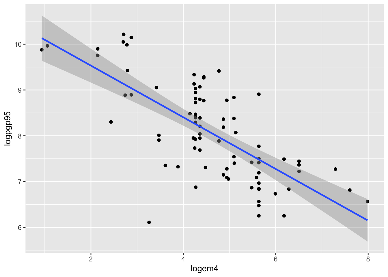

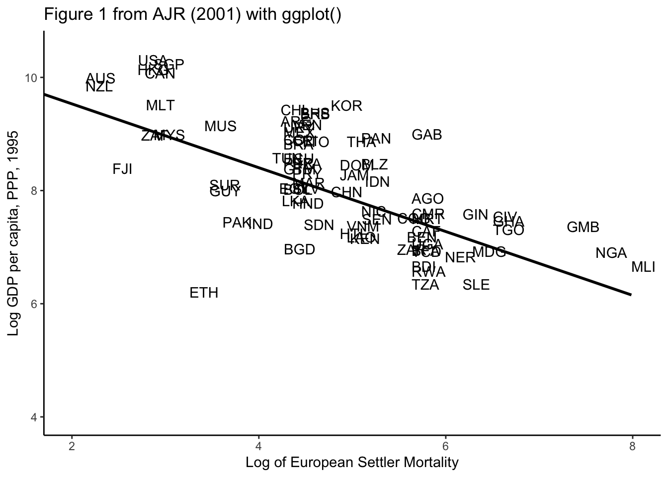
Advanced:

figure <- ggplot(data, aes(x = logem4, y=logpgp95)) + #Settler mortality and GDP per Cap
  #geom_point() + #if we want to use points
  geom_text(aes(label=data[,1]),hjust=0, vjust=0) + #if we want the country names as points
  geom_smooth(color="black",method="lm", se=FALSE) + 
  theme_classic()+ 
  coord_cartesian(xlim=c(2,8), ylim=c(4,10.5)) + 
  labs(
    title="Figure 1 from AJR (2001) with ggplot()",
    x="Log of European Settler Mortality", 
    y="Log GDP per capita, PPP, 1995"
    )
figure

`geom_smooth()` using formula 'y ~ x'

Warning: Removed 82 rows containing non-finite values (stat_smooth).

Warning: Removed 82 rows containing missing values (geom_text).

16.11.2023 Time Series

Time Series

Panel Data

ggplot